Recreating Manfred Mohr's Cubic Limit Series with Effect

February 8, 2025 · fp and typescript

This post walks through the process of recreating Manfred Mohr's iconic artwork Cubic Limit, P-161 with TypeScript and Effect using a fully functional rendering pipeline.

Shown below is a replica of P-161 (six edges), originally part of a 13-piece plotter drawing series from 1975, which is widely recognized as a pioneering work in algorithmic art.

Clone the Repository

The full source code that produces this image is available here. It is an Effect-based adaptation of graphics-ts with support for 3D rendering. Clone it with:

git clone git@github.com:tetsuo/cubic-limit.git

The repository also includes a version of P-197, but this post will focus solely on P-161.

Cube Vertices & Edges

We'll work with a type Vec to hold [x, y, z] coordinates.

type Vec = NonEmptyReadonlyArray<number>
// e.g. [x, y, z]

A unit cube (scaled from -1 to +1) has 8 vertices:

const cubePoints: NonEmptyReadonlyArray<Vec> = [
  [-1, -1, -1],
  [ 1, -1, -1],
  [ 1,  1, -1],
  [-1,  1, -1],
  [-1, -1,  1],
  [ 1, -1,  1],
  [ 1,  1,  1],
  [-1,  1,  1],
]

It has 12 edges. We can index them by grouping bottom edges, top edges, and vertical edges. For each i in 0..3, we build three edges:

const getEdges = (i: number): NonEmptyReadonlyArray<Vec> => [
  [i, (i + 1) % 4],
  [i + 4, ((i + 1) % 4) + 4],
  [i, i + 4],
]

Combining all i values yields 12 edges. Each edge is a pair of indices into cubePoints.

Cube Configurations

Mohr's piece shows a 31×31 grid of partially drawn cubes. Each cube is unique and displayed with exactly six edges (n = 6). To represent this mathematically:

Label each of the cube's 12 edges as a bit in a 12-bit integer.
Turning on an edge = setting the corresponding bit to 1.

This means each valid cube configuration is a 12-bit number with exactly six bits set to 1.

How many such configurations exist? Exactly 924, as determined by the formula C(12, 6) = 924.

These numbers correspond to OEIS sequence A023688, which lists integers with six 1s in their binary representation. Within the 12-bit range, the sequence starts at 63 (binary 000000111111) and ends just under 4095 (binary 111111111111):

63    -- 000000111111
95    -- 000001011111
111   -- 000001101111
.
.
4032  -- 111111000000

Generating All 12-Bit Numbers with Six 1s

To iterate through all 12-bit integers that have exactly six bits set, I turned to a classic resource: Bit Twiddling Hacks. At the bottom of that page is the code to compute the lexicographically next bit permutation:

import { pipe } from 'effect/Function'

const nextNumber = (v: number) =>
  pipe(
    (v | (v - 1)) + 1,
    t => t | ((((t & -t) / (v & -v)) >> 1) - 1)
  )

This function finds the next integer with the same number of bits set. For example, if v has exactly 6 bits set, it will produce the next integer that also has 6 bits set.

With it, we can now accumulate all valid edge combinations:

import { unfold } from 'effect/Array'
import { none, some } from 'effect/Option'

const seq: number[] = unfold(63, a => a < 4095 ? some([a, nextNumber(a)]) : none()
)
// => [63, 95, 111, 119, ... 4032, etc.]

Each integer in seq encodes a unique cube with exactly 6 edges, totaling 924 configurations.

Representing Geometry

Shape

The Shape type is originally defined in the purescript-drawing library:

type Point = { x :: Number, y :: Number }

data Shape
  = Path Boolean (List Point)
  | Composite (List Shape)

For our implementation, we borrow the graphics-ts port of Shape with one critical change: our points will be multi-dimensional. Therefore, the Point type will alias to Vec:

type Point = Vec

const point = (x: number, y: number, z: number): Point => [x, y, z]

So a Shape is a union of Path and Composite, meaning it can represent one of two things. In TypeScript, this translates to:

type Shape = Path | Composite

Path

A Path is a chunk of points connected by lines, plus a boolean to indicate whether the path is closed (i.e., the last point connects back to the first):

import { Chunk } from '@effect/data/Chunk'

interface Path {
  readonly _tag: 'Path'
  readonly closed: boolean
  readonly points: Chunk<Point>
}

We define two constructors, path and closed, which take a Foldable—an abstraction for collections that can be reduced to a single value (e.g., an Array). We also define a Monoid instance for Path, which combines two paths by concatenating their points and checking if either path is closed.

import { MonoidSome } from '@effect/typeclass/data/Boolean'
import { constant } from 'effect/Function'
import { fromSemigroup, Monoid, struct } from '@effect/typeclass/Monoid'
import { make } from '@effect/typeclass/Semigroup'
import { Foldable } from '@effect/typeclass/Foldable'
import { Kind, TypeLambda } from 'effect/HKT'
import { Chunk, append, appendAll, empty } from '@effect/data/Chunk'

// Constructors

const closed =
  <F extends TypeLambda>(F: Foldable<F>): ((fa: Kind<F, unknown, unknown, unknown, Point>) => Path) =>
  fa =>
    F.reduce(fa, monoidPath.empty, (b, a) => ({
      _tag: 'Path',
      closed: true,
      points: append(b.points, a),
    }))

const path =
  <F extends TypeLambda>(F: Foldable<F>): ((fa: Kind<F, unknown, unknown, unknown, Point>) => Path) =>
  fa =>
    F.reduce(fa, monoidPath.empty, (b, a) => ({
      _tag: 'Path',
      closed: false,
      points: append(b.points, a),
    }))

// Monoid instance

const monoidPath: Monoid<Path> = struct({
  _tag: fromSemigroup<'Path'>(make(constant('Path')), 'Path'),
  closed: MonoidSome,
  points: fromSemigroup(make<Chunk<Point>>(appendAll), empty()),
})

Here, the monoidPath combines two Path objects by merging their point arrays. The MonoidSome ensures that if any of the paths are closed, the result is also considered closed.

Composite

The other variant of Shape is Composite, which basically serves as a container for multiple Shapes:

interface Composite {
  readonly _tag: 'Composite'
  readonly shapes: ReadonlyArray<Shape>
}

const composite = (shapes: ReadonlyArray<Shape>): Composite => ({
  _tag: 'Composite',
  shapes,
})

Constructing a Full Cube

Bringing it all together, here's how we can define a full cube (all 12 edges visible) as a Composite of 12 paths:

import { pipe } from 'effect/Function'
import { flatMap, map, range } from 'effect/Array'
import { Foldable } from '@effect/typeclass/data/Array'
import { tuple } from 'effect/Data'
import * as S from './Shape'

const path = S.path(Foldable)

const cubeShape = S.composite(
  pipe(
    range(0, 3),
    flatMap(i =>
      pipe(
        getEdges(i),
        map(ix =>
          path(
            pipe(
              tuple(points[ix[0]], points[ix[1]]),
              map(vec => S.point(vec[0], vec[1], vec[2]))
            )
          )
        )
      )
    )
  )
)

Cube as a Composite of Paths

The cubeShape structure represents the cube's 12 edges as pairs of points in 3D space. Each point is a 3D vector[x, y, z], and each edge is defined by two such points:

[
  [
    [-1, -1, -1], // Start point
    [1, -1, -1],  // End point
  ],
  [
    [-1, -1, 1],
    [1, -1, 1],
  ],
  ... (12 pairs in total)
]

Each innermost array defines a Point, represented by its x, y, and z coordinates.
Each array containing point tuples describes a Path, which corresponds to a single edge of the cube.
12 paths are grouped together into a Composite.

Toggling Edges to Form Partial Cubes

Since Mohr's P-161 selectively displays only 6 edges of the cube, we need a way to toggle edges (paths) on/off. We can do that by passing in a predicate that checks if an edge is active.

import { Predicate } from 'effect/Predicate'

const cubeShape = (shouldDrawEdge: Predicate<number>): S.Composite =>
  S.composite(
    pipe(
      range(0, 3),
      flatMapArray(i =>
        pipe(
          getEdges(i),
          mapArray((ix, j) =>
            path(
              shouldDrawEdge(i + j * 4)
                ? pipe(
                    tuple(points[ix[0]], points[ix[1]]),
                    mapArray(vec => S.point(vec[0], vec[1], vec[2]))
                  )
                : [] // ← empty when shouldDrawEdge(edge) returns false
            )
          )
        )
      )
    )
  )

We define a utility isBitSet, returning true if a given bit is set in n:

const isBitSet = (n: number) => (index: number) =>
  Boolean(n & (1 << index))

Then we build a function cubeFromNumber that uses isBitSet to determine which edges should be drawn:

import { flow } from 'effect/Function'

const cubeFromNumber = flow(isBitSet, cubeShape)

If n has bits 3, 5, 8, 10, etc., turned on, only those edges of the cube are visible.

For example, calling cubeFromNumber(63) (binary 000000111111) will omit edges 0 through 5 and include edges 6 through 11, producing a half-formed cube.

Generating All Cube Shapes

Finally, we can list all 924 cube shapes corresponding to n = 6 by:

Generating all 12-bit numbers with 6 bits set (using unfold and nextNumber).
Mapping each integer to a Shape with cubeFromNumber.

import { none, some } from 'effect/Option'
import { map, unfold } from 'effect/Array'

const cubes: Composite[] = pipe(
  unfold(63, a => (a < 4095 ? some([a, nextNumber(a)]) : none())),
  map(cubeFromNumber)
)

// cubes is now an array of 924 partial cube shapes

Representing Styles & Transformations

Drawing

Next, we define a new type that captures what we want to do with shapes—whether to fill them, outline them, apply transformations, or clip:

type Drawing =
  | { _tag: 'Translate'; translateX: number; translateY: number; translateZ: number; drawing: Drawing }
  | { _tag: 'Rotate'; rotateX: Angle; rotateY: Angle; rotateZ: Angle; drawing: Drawing }
  | { _tag: 'Scale'; scaleX: number; scaleY: number; scaleZ: number; drawing: Drawing }
  | { _tag: 'Many'; drawings: ReadonlyArray<Drawing> }
  | { _tag: 'Clipped'; shape: Shape; drawing: Drawing }
  | { _tag: 'Fill'; shape: Shape; style: FillStyle }
  | { _tag: 'Outline'; shape: Shape; style: OutlineStyle }

A Drawing acts like a scene graph, where transformations (Scale, Rotate, Translate) can be nested around shapes.

To convert a Shape into a Drawing, we use one of three options: Clipped, Fill, or Outline.

Outline

The Outline variant in Drawing represents shapes rendered with an outline. The function outline constructs an outlined shape with a given OutlineStyle (color, lineWidth, etc.):

const outline: (shape: Shape, style: OutlineStyle) => Drawing = (shape, style) => ({
  _tag: 'Outline',
  shape,
  style,
})

Applying Outlines to Cubes:

import * as D from './Drawing'

const lineColor = D.outlineColor(white)

const cubeLineStyle = D.monoidOutlineStyle.combine(lineColor, D.lineCap('round'))

const cubes = pipe(
  unfold(63, a => (a < 4095 ? some([a, nextNumber(a)]) : none())),
  map(flow(cubeFromNumber, cube => D.outline(cube, cubeLineStyle)))
)

Fill

Just like Outline defines shapes with an outline, the Fill variant in Drawing represents shapes rendered with a fill. The function fill creates a filled shape using a specified FillStyle.

const fill: (shape: Shape, style: FillStyle) => Drawing = (shape, style) => ({
  _tag: 'Fill',
  shape,
  style,
})

Drawing Background:

import { Foldable } from '@effect/typeclass/data/Array'
import { hsl } from './Color'
import * as S from './Shape'
import * as D from './Drawing'

const closed = S.closed(Foldable)

const drawBackground = ({ width, height }: Size, bgColor: Color): D.Drawing =>
  D.fill(
    closed([
      [0, 0, 0],
      [width, 0, 0],
      [width, height, 0],
      [0, height, 0],
    ]),
    D.fillStyle(bgColor)
  )

Many

The Many variant allows combining multiple Drawing objects into a single composition, conceptually just a list.

const many: (drawings: ReadonlyArray<Drawing>) => Drawing = drawings => ({
  _tag: 'Many',
  drawings,
})

Drawing a Grid Of Lines:

import { map, range } from 'effect/Array'
import { white } from './Color'
import * as D from './Drawing'

const lineColor = D.outlineColor(white)

// drawLines creates evenly spaced vertical or horizontal lines by dividing
// the given height into n segments and mapping them into outlined paths.
const drawLines = (n: number, height: number, vertical: boolean): D.Drawing => {
  const size = height / n
  return D.many(
    pipe(
      range(1, n - 1),
      map(i =>
        D.outline(
          path(
            vertical
              ? [
                  [i * size, 0, 0],
                  [i * size, height, 0],
                ]
              : [
                  [0, i * size, 0],
                  [height, i * size, 0],
                ]
          ),
          lineColor
        )
      )
    )
  )
}

Translate / Scale / Rotate

The each of the following constructors wraps a Drawing and includes X, Y, Z parameters to translate, rotate, or scale whatever is inside.

const translate = (
  translateX: number,
  translateY: number,
  translateZ: number,
  drawing: Drawing
): Drawing => ({ _tag: 'Translate', translateX, translateY, translateZ, drawing })

const scale = (
  scaleX: number,
  scaleY: number,
  scaleZ: number,
  drawing: Drawing
): Drawing => ({ _tag: 'Scale', scaleX, scaleY, scaleZ, drawing })

const rotate = (
  rotateX: Angle,
  rotateY: Angle,
  rotateZ: Angle,
  drawing: Drawing
): Drawing => ({ _tag: 'Rotate', rotateX, rotateY, rotateZ, drawing })

Rotating, Scaling, and Positioning Cubes:

import { map, unfold } from 'effect/Array'
import { none, some } from 'effect/Option'
import * as D from './Drawing'
import * as S from './Shape'

// drawCubes generates a grid of outlined cubes.
const drawCubes = (numCells: number, cellSize: number): D.Drawing => {

  // translateCube positions each cube based on its row/column index.
  const translateCube = (drawing: D.Drawing, i: number): D.Drawing => {
    const translateX = cellSize * (numCells - Math.floor(i / numCells) - 0.5)
    const translateY = cellSize * (0.5 + (i % numCells))
    return D.translate(translateX, translateY, 0, drawing)
  }

  // Scale factor compensates for the original cube points being doubled.
  const scaleFactor = cellSize / 5

  return D.rotate(
    S.degrees(30),
    S.degrees(-60),
    S.degrees(0),
    D.scale(
      scaleFactor,
      scaleFactor,
      1, // Z remains unchanged.
      D.many(
        pipe(
          unfold(63, a => (a < 4095 ? some([a, nextNumber(a)]) : none())),
          map(flow(cubeFromNumber, cube => D.outline(cube, cubeLineStyle))),
          map(translateCube)
        )
      )
    )
  )
}

Drawing P-161

Finally, we end up with a Drawing that visually represents Cubic Limit, P-161 in its entirety 🎉

const drawP161 = (size: Size, bgColor: Color): D.Drawing => {
  const numCells = 31
  const cellSize = size.width / numCells

  const background = drawBackground(size, bgColor)

  const lines = D.many([
    drawLines(numCells, size.width, false),
    drawLines(numCells, size.height, true)
  ])

  const cubes = drawCubes(numCells, cellSize)

  return D.many([background, lines, cubes])
}

The Art of Rendering Cubes and Generating Side Effects

Today's technology lets us render 3D shapes with a few lines of code, but Mohr's process was far more hands-on. The Cubic Limit series was originally drawn using a Benson 1284 flatbed plotter.

Manfred Mohr and Estarose Wolfson

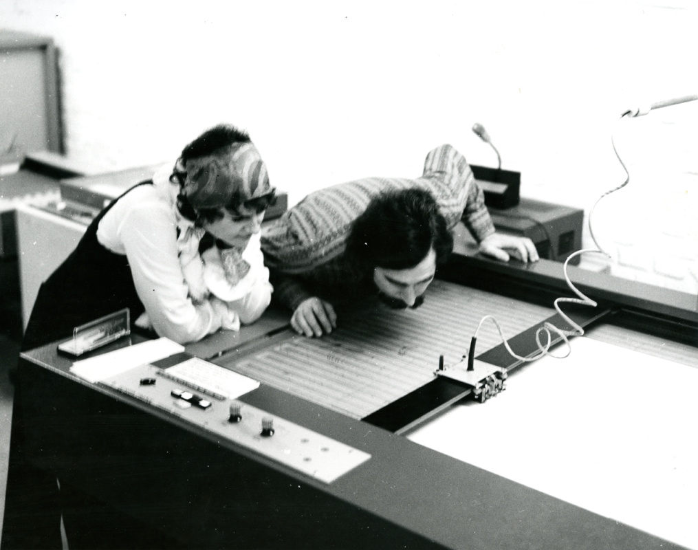
Manfred Mohr and Estarose Wolfson look at the Benson plotter in the Centre de Calcul de la Météorologie Nationale, 1971 / © Manfred Mohr (Source)

Mohr developed his algorithms on a CDC 6400 mainframe with Fortran IV, storing his code on punch cards. With these programs, he transformed and projected cubes onto a 2D plane, ultimately generating low-level instructions for the plotter.

While details about this plotter's proprietary language—likely called Benson Graphic Language (BGL)—are scarce, it probably shared similarities with Hewlett Packard's HP-GL. For example, drawing a rectangle in HP-GL might look like this:

SP1          // Select pen 1
PU 0,0       // Pen up (move without drawing)
PD 100,0     // Pen down (start drawing)
PD 100,100
PD 0,100
PD 0,0
PU           // Pen up (stop drawing)

Note that these plotter languages somewhat resemble the Canvas API. For example:

PU (Pen Up) corresponds to moveTo.
PD (Pen Down) corresponds to lineTo.

Here is a basic rectangle-drawing example:

const canvas = document.getElementById('myCanvas');
const ctx = canvas.getContext('2d');

ctx.beginPath();
ctx.moveTo(0, 0);
ctx.lineTo(100, 0);
ctx.lineTo(100, 100);
ctx.lineTo(0, 100);
ctx.closePath();
ctx.stroke();

In essence, from Mohr's era to today's digital canvas, the process remains the same: first, you model your art in code, and then you generate the instructions that bring it to life.

Modern techniques, especially in functional programming, explicitly enforce this separation. You often end up with:

A declarative model that specifies what to do
An interpreter that connects this model to stateful, effectful APIs

The Drawing sum type describes the semantics of a domain specific language (DSL) for creating vector graphics, keeping the model separate from side effects. This separation allows the same underlying logic to be used for rendering to a canvas, exporting to PostScript, or even controlling a physical plotter. Our plan is to eventually integrate it with the Canvas API, and ultimately generate canvas commands as a side effect.

Interpreting Geometry

Before we proceed, we must address a key limitation: the Canvas API only supports 2D coordinates (i.e., X and Y), not 3D.

To work around this constraint, we'll begin by implementing a simplified version of the CanvasPath API—similar to Path2D—but tailored to handle 3D coordinates.

Path3D

type Path3D = ReadonlyArray<ReadonlyArray<Point>>

Path3D is an intermediate representation that transforms our high-level Shape definitions into a format more suitable for applying transformations and rendering. Essentially, it flattens a shape into an array of subpaths, where each subpath is a sequence of 3D points ([x, y, z]).

Converting a Shape to Path3D

The helper function fromShape performs this conversion:

const fromShape: (shape: Shape) => Path3D = shape => {
  switch (shape._tag) {
    case 'Composite':
      // For composites, recursively process each child shape and concatenate the results.
      return shape.shapes.flatMap(fromShape)
    case 'Path':
      // For a simple path, convert its points into a subpath.
      return pipe(
        toReadonlyArray(shape.points),
        matchLeft({
          onEmpty: empty,
          onNonEmpty: (head, tail) =>
            pipe(
              tail,
              map(lineTo),
              reduce(moveTo(head)([]), (acc, f) => f(acc)),
              path => (shape.closed ? closePath(path).slice(0, -1) : path)
            ),
        })
      )
  }
}

For a Composite, fromShape simply calls fromShape on each sub-shape and concatenates the resulting Path3D arrays.

For a Path, fromShape breaks the points into line segments (via moveTo and lineTo). If closed is true, it calls closePath, making the last point connect to the first.

Path3D Combinators: moveTo, lineTo, closePath

These functions implement the path-drawing algorithm:

moveTo

Begins a new subpath at the specified point (if the point is finite).

const moveTo = (point: Point) => (path: Path3D): Path3D =>
  isPointFinite(point)
    ? // Create a new subpath with the specified point.
      append(path, [point])
    : path

lineTo

Extends the current subpath by connecting the last point to the new point.

const lineTo = (point: Point) => (path: Path3D): Path3D =>
  isPointFinite(point)
    ? isNonEmptyReadonlyArray(path)
      ? // Connect the last point in the subpath to the given point.
        pipe(path, modifyNonEmptyLast(append(point)))
      : // If path has no subpaths, ensure there is a subpath.
        moveTo(point)(path)
    : path

closePath

Closes the current subpath by connecting its last point back to the first.

const closePath = (path: Path3D): Path3D => {
  // Do nothing if path has no subpaths.
  if (!isNonEmptyReadonlyArray(path)) {
    return path
  }

  const cur = lastNonEmpty(path)

  // Do nothing if the last path contains a single point.
  if (!(isNonEmptyReadonlyArray(cur) && cur.length > 1)) {
    return path
  }

  const end = lastNonEmpty(cur)
  const start = cur[0]

  // Do nothing if both ends are the same point.
  if (end[0] === start[0] && end[1] === start[1] && end[2] === start[2]) {
    return path
  }

  // Mark the last path as closed adding a new subpath whose first point
  // is the same as the previous subpath's first point.
  return append(setNonEmptyLast(append(cur, start) as ReadonlyArray<Point>)(path), [start])
}

Transformation Matrices

Rendering a 3D scene onto a 2D canvas typically involves a series of steps—applying model, view, and projection matrices, performing perspective division, etc. In our case, however, we only require model transformations—positioning, scaling, and rotating each individual cube.

Mat

These transformations are typically encoded in 4×4 matrices when dealing with 3D points. We can define a matrix type Mat as follows:

type Mat = NonEmptyReadonlyArray<Vec>

Common 3D Transforms

A standard 4×4 transform matrix looks like this:

[sx   0    0    tx]
[0    sy   0    ty]
[0    0    sz   tz]
[0    0    0    1 ]

sx, sy and sz control scaling on each axis.
tx, ty and tz control translation along each axis.
Off-diagonal terms can encode rotation and other transformations.

For example, a pure scale transformation might look like this:

const scale = (v: Vec): Mat => [
  [v[0], 0,    0,    0],
  [0,    v[1], 0,    0],
  [0,    0,    v[2], 0],
  [0,    0,    0,    1],
]

Likewise, a rotation about the X-axis by some angle can be represented as:

const sin = (deg: number) => Math.sin((deg * Math.PI) / 180)
const cos = (deg: number) => Math.cos((deg * Math.PI) / 180)

const rotateX = (angle: number): Mat => [
  [1, 0,           0,          0],
  [0, cos(angle),  sin(angle), 0],
  [0, -sin(angle), cos(angle), 0],
  [0, 0,           0,          1],
]

Combining Multiple Transforms

Often we need to combine several transformations (e.g. translate first, then rotate, then scale). In matrix math, combining transformations is done by matrix multiplication:

declare function mul(y: Mat): (x: Mat) => Mat

pipe(
  identity, // The 4×4 identity matrix (no transformation)
  mul(translate([10, 0, 0])),
  mul(rotateX(45)),
  mul(rotateY(30)),
  mul(scale([2, 2, 2]))
)

The final result is a single 4×4 matrix encoding all these operations in the correct order. When you apply that matrix to a point [x, y, z, 1], it performs the entire sequence of transformations—translation, then rotation on X, then rotation on Y, then scaling.

Reminder: Matrix multiplication is not commutative. The order you multiply matters.

Semigroup & Monoid for Matrices

Because matrix multiplication is associative, we can define a Semigroup for Mat:

import { Semigroup, make } from '@effect/typeclass/Semigroup'

// semigroupMat: given two matrices x and y, how do we combine them?
const semigroupMat: Semigroup<Mat> = make((x, y) => {
  // matrix multiplication logic
})

And from that Semigroup, we get a Monoid by adding the identity matrix (which leaves any vector unchanged):

import { Monoid, fromSemigroup } from '@effect/typeclass/Monoid'

const monoidMat: Monoid<Mat> = fromSemigroup(
  semigroupMat,
  identity // 4×4 identity matrix
)

This way, we can compose an array of transformations neatly:

import { monoidMat } from './Mat'

const combined = monoidMat.combineAll([
  translate([5, 0, 0]),
  scale([2, 2, 2]),
  rotateZ(90),
])

Dot Products & Matrix Multiplication

Under the hood, matrix multiplication boils down to computing dot products between rows of the first matrix and columns of the second:

const dot =
  (b: Vec) =>
  (a: Vec) =>
    pipe(zipWith(a, b, multiply), reduce(0, sum))

const col: (n: number) => (m: Mat) => Vec = n => map(unsafeGet(n))

const transpose = (m: Mat): Mat =>
  pipe(
    headNonEmpty(m),
    map((_, i) => col(i)(m))
  )

const mul = (x, y) =>
  pipe(
    map(transpose(y), dot),
    // then for each row in x, apply the dotted function
    fab => map(x, ar => map(fab, f => f(ar)))
  )

When multiplying C=A×B, each entry (i,j) in C is the dot product of row i from A with column j from B.

Applying 3D Transformations

The toCoords helper function takes a Shape, extracts its constituent subpaths, applies a transformation matrix, and outputs the final coordinates to be sent to the Canvas API.

const toCoords = (shape: Shape, transform: Mat): ReadonlyArray<ReadonlyArray<Point>> =>
  pipe(
    // 1. Convert the shape into an array of subpaths.
    fromShape(shape),
    // 2. Attempt to convert each subpath into a NonEmpty array.
    map(validateNonEmpty),
    // 3. Filter out any empty subpaths.
    compactArray,
    // 4. Append a 1 to each coordinate for homogeneous transformation.
    map(map(append(1))),
    // 5. Multiply each coordinate by the transformation matrix.
    map(mul(transform))
  )

The Render Service

Now that everything is in place, let's define the Render service as a tagged interface that encapsulates methods mirroring those of the native CanvasRenderingContext2D (e.g. lineTo, moveTo, fill, stroke, etc.).

Here's the full definition:

class Render extends Tag('Render')<
  Render,
  {
    readonly lineTo: (point: Vec) => Micro<void>
    readonly moveTo: (point: Vec) => Micro<void>
    readonly fill: (fillRule?: CanvasFillRule) => Micro<void>
    readonly clip: (fillRule?: CanvasFillRule) => Micro<void>
    readonly stroke: () => Micro<void>
    readonly beginPath: () => Micro<void>
    readonly closePath: () => Micro<void>
    readonly save: () => Micro<void>
    readonly restore: () => Micro<void>
    readonly setFillStyle: (style: string) => Micro<void>
    readonly setStrokeStyle: (style: string) => Micro<void>
    readonly setLineWidth: (width: number) => Micro<void>
    readonly setLineCap: (cap: D.LineCap) => Micro<void>
    readonly setLineJoin: (join: D.LineJoin) => Micro<void>
  }
>() {}

Producing Render Effect

The function renderDrawing is our core interpreter for the Drawing DSL. It takes a Drawing and recursively transforms it into a series of canvas commands, while internally maintaining a transformation matrix that accumulates and applies all transformations.

const renderDrawing = (d: D.Drawing): Micro<void, never, Render> =>
  service(Render).pipe(
    andThen(c => {
      // Wrap an operation with save/restore for context isolation.
      const withContext = (fa: Micro<void>) =>
        pipe(
          c.save(),
          andThen(() => fa),
          andThen(c.restore)
        )

      const applyStyle: <A>(o: Option<A>, f: (a: A) => Micro<void>) => Micro<void> = (fa, f) =>
        isSome(fa) ? f(fa.value) : success

      // Render a single sub-path using moveTo and lineTo.
      const renderSubPath: (subPath: ReadonlyArray<Point>) => Micro<void> = matchLeft({
        onEmpty: () => success,
        onNonEmpty: (head, tail) =>
          pipe(
            c.moveTo(head),
            andThen(() => forEach(tail, c.lineTo, { discard: true }))
          ),
      })

      // Convert a Shape to a Path3D using fromShape, transform it, then render each sub-path.
      const renderShape = (shape: Shape, transform: Mat) =>
        forEach(toCoords(shape, transform), renderSubPath, { discard: true })

      // The recursive interpreter that handles all variants of Drawing.
      const go: (drawing: D.Drawing, transform: Mat) => Micro<void> = (d, t) => {
        switch (d._tag) {
          case 'Many':
            return forEach(d.drawings, d => go(d, t), { discard: true })
          case 'Scale':
            return go(d.drawing, semigroupMat.combine(t, scale([d.scaleX, d.scaleY, d.scaleZ])))
          case 'Rotate':
            return go(
              d.drawing,
              semigroupMat.combineMany(t, [
                rotateZ(angle(d.rotateZ)),
                rotateY(angle(d.rotateY)),
                rotateX(angle(d.rotateX)),
              ])
            )
          case 'Translate':
            return go(
              d.drawing,
              semigroupMat.combine(t, translate([d.translateX, d.translateY, d.translateZ]))
            )
          case 'Outline':
            return withContext(
              pipe(
                applyStyle(d.style.color, flow(Color.toCss, c.setStrokeStyle)),
                andThen(() => applyStyle(d.style.lineWidth, c.setLineWidth)),
                andThen(() => applyStyle(d.style.lineCap, c.setLineCap)),
                andThen(() => applyStyle(d.style.lineJoin, c.setLineJoin)),
                andThen(c.beginPath),
                andThen(() => renderShape(d.shape, t)),
                andThen(c.stroke)
              )
            )
          case 'Fill':
            return withContext(
              pipe(
                applyStyle(d.style.color, flow(Color.toCss, c.setFillStyle)),
                andThen(c.beginPath),
                andThen(() => renderShape(d.shape, t)),
                andThen(() => c.fill())
              )
            )
          case 'Clipped':
            return withContext(
              pipe(
                c.beginPath(),
                andThen(() => renderShape(d.shape, t)),
                andThen(() => c.clip()),
                andThen(() => go(d.drawing, t))
              )
            )
        }
      }
      return go(d, identity)
    })
  )

Transformation Composition

The recursive function go walks through a Drawing, updating the transform matrix (with operations like Scale, Rotate, and Translate) as it recurses through nested drawings.

Style and Context Management

For instructions like Outline and Fill, the function saves the canvas state, applies style settings, begins a new path, renders the shape, executes the appropriate drawing command (stroke or fill), and finally restores the canvas state.

Sub-Path Rendering

The helper renderSubPath converts a sub-path (a list of 3D points) into the corresponding canvas calls (moveTo for the first point, followed by lineTo for subsequent points).

Wiring Up the Real Canvas

The final step is the render function, which "plugs in" a real CanvasRenderingContext2D implementation by providing a concrete instance of the Render service. This function builds the effect (from renderDrawing) and then supplies a real implementation that calls the actual Canvas API:

const render = (d: D.Drawing, ctx: CanvasRenderingContext2D): Micro<void, never, never> =>
  provideService(renderDrawing(d), Render, {
    fill(fillRule) {
      ctx.fill(fillRule)
      return succeed(undefined)
    },
    clip(fillRule) {
      ctx.clip(fillRule)
      return succeed(undefined)
    },
    setFillStyle(style: string) {
      ctx.fillStyle = style
      return succeed(undefined)
    },
    setStrokeStyle(style: string) {
      ctx.strokeStyle = style
      return succeed(undefined)
    },
    setLineWidth(width: number) {
      ctx.lineWidth = width
      return succeed(undefined)
    },
    setLineJoin(join: D.LineJoin) {
      ctx.lineJoin = join
      return succeed(undefined)
    },
    setLineCap(cap: D.LineCap) {
      ctx.lineCap = cap
      return succeed(undefined)
    },
    stroke() {
      ctx.stroke()
      return succeed(undefined)
    },
    save() {
      ctx.save()
      return succeed(undefined)
    },
    restore() {
      ctx.restore()
      return succeed(undefined)
    },
    lineTo(p) {
      ctx.lineTo(p[0], p[1])
      return succeed(undefined)
    },
    moveTo(p) {
      ctx.moveTo(p[0], p[1])
      return succeed(undefined)
    },
    beginPath() {
      ctx.beginPath()
      return succeed(undefined)
    },
    closePath() {
      ctx.closePath()
      return succeed(undefined)
    },
  })

Putting It All Together

Finally, the renderTo function ties everything together. It retrieves the canvas element, adjusts its size for the device pixel ratio, gets the 2D context, and runs the rendering effect:

const renderTo = (f: (size: Size) => Drawing, canvasId: string): void =>
  pipe(
    // 1. Obtain a canvas.
    getCanvasElementById(canvasId),
    andThen(canvas => {
      // 2. Scale the canvas according to the device pixel ratio.
      const rect = canvas.getBoundingClientRect()
      return dpr.pipe(
        andThen(dpr => {
          canvas.width = rect.width * dpr
          canvas.height = rect.height * dpr
          canvas.style.width = `${rect.width}px`
          canvas.style.height = `${rect.height}px`
          return pipe(
            // 3. Get the 2D context.
            getContext2D(canvas),
            andThen(ctx => {
              ctx.scale(dpr, dpr)
              // 4. Compute the Drawing by calling f(size) and render it on the context.
              return render(f({ height: canvas.height / dpr, width: canvas.width / dpr }), ctx)
            })
          )
        })
      )
    })
  ).pipe(runSync) // 5. Perform the side-effect on the canvas.

Rendering P-161

const renderP161 = (canvasId: string, bgColor: string) =>
  renderTo(size => drawP161(size, hex(bgColor)), canvasId)